One of the trend on developer is AI and machine learing, and I think most of engineer, like me, are trying to going into this field. To start on machine learning, we need a knowledge about data analysis, and for that we have to remind statistics, which we suffered when we are a student.

Linear Regression?

Linear Regression is one way to find relation between variable, with given dataset. This theory has been more than a hundread years, but it is still broadly used and printed in most of machine learning text books.

Linear Regression tries to make a linear line like y = Ax + B which closely match values in data. It is the way to figure out A and B value from predictor value x and target value y. There also can be more than one variable in predict value, it is called as ‘Multiple Linear Regression’, and then it will have form like y = A1x + A2x + A3x + A4x + ... + B. Similarly, first case with single depandant value are being called as ‘Single Linear Regression’. I’ll focus looking in this case on this post.

Before starting

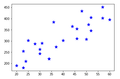
I’ll use numpy, but try not to use other python modules for machine learning this time, such as pandas or scikit-learn, to look on detail process of this. I prepared simple dataset for test. Here are information about ‘age’, ‘blood fat’ of 25 anonymous people. You can find this, and some other dataset in http://people.sc.fsu.edu/~jburkardt/datasets/regression/regression.html

Implementation

Let’s think about the first case, with single dependant variable. I’ll look on how age is related with blood fat.

{% highlight python %} {% raw %} import csv import matplotlib.pyplot as plt

csv_file = open(‘data.csv’, ‘r’) reader = csv.reader(csv_file) x = [] # age y = [] # blood fat

for value in reader: x.append(value[1]) y.append(value[2])

plt.scatter(x, y, color = “b”, marker = “*”, s = 100) plt.show() {% endraw %} {% endhighlight %}

You could find result like below.

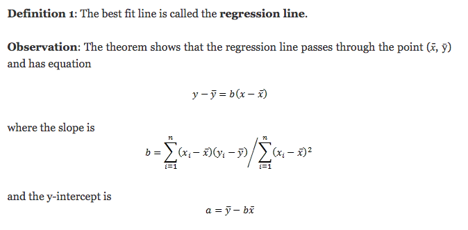
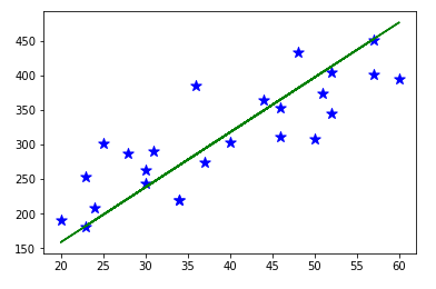
Now, we need to think about how to get proper point to make a linear line to cover these points, which called regression line. The best fit line is the line for which the sum of the distances between each of data points and the line is as small as possible. For this, I’ll make an implementation of Least square method.

This is the implementation for this logic. I used numpy for this to make calculation in list more simple.

{% highlight python %} {% raw %}

input ‘x_arr’, ‘y_arr’ is np.array

def least_square_method(x_arr, y_arr): x_mean, y_mean = np.mean(x_vec), np.mean(y_vec) set_size = np.size(x_vec)

numerator = np.sum(y_vec*x_vec - set_size*y_mean*x_mean)
denominator = np.sum(x_vec*x_vec - set_size*x_mean*x_mean)

b_1 = numerator / denominator
b_0 = y_mean - b_1*x_mean

return(b_0, b_1)

{% endraw %} {% endhighlight %}

Now let’s look on main code.

{% highlight python %} {% raw %} def main(): x_vector = np.array(x) y_vector = np.array(y) b = least_square_method(x_vector, y_vector) y_prediction = b[0] + b[1] * x_vector

plt.scatter(x_vector, y_vector, color = "b", marker = "*", s = 100)
plt.plot(x_vector, y_prediction, color = "g")

plt.show()

{% endraw %} {% endhighlight %}

Let’s look on the result.

Next time I’ll look on Multiple Linear Regression, and other theories about regression.