As I wrote in previous post, most dataset in real world are not clean. They are usually messed up, incompatible(ex:’-1’ is included in data which defines people’s age), and some of are missing. These kind of dataset will mostly cause error, or return wrong result when you just put on your elaborated logic. That’s why you need to concern pre-process before researching it.
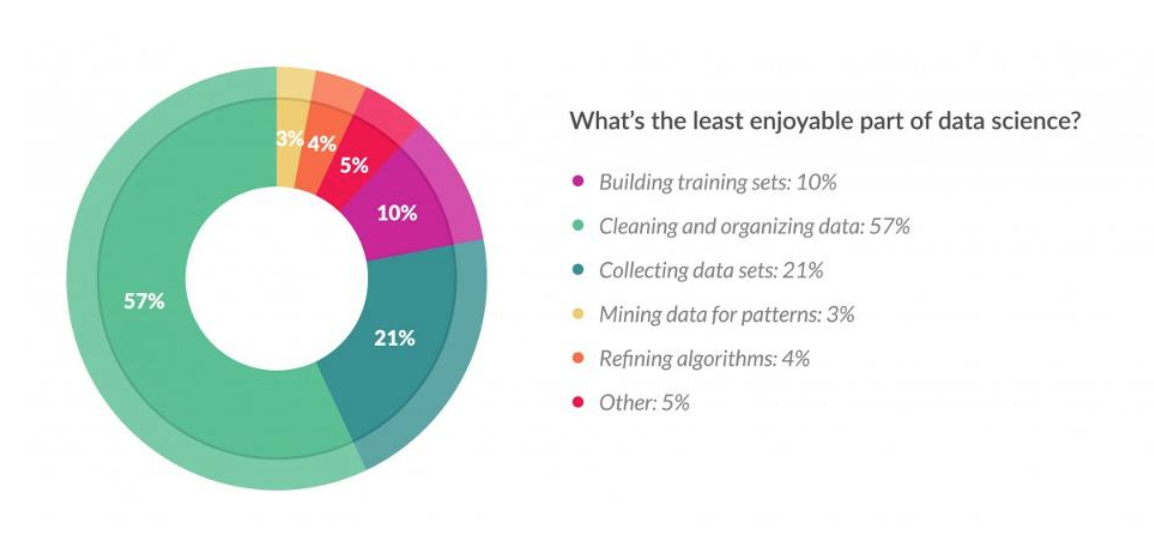
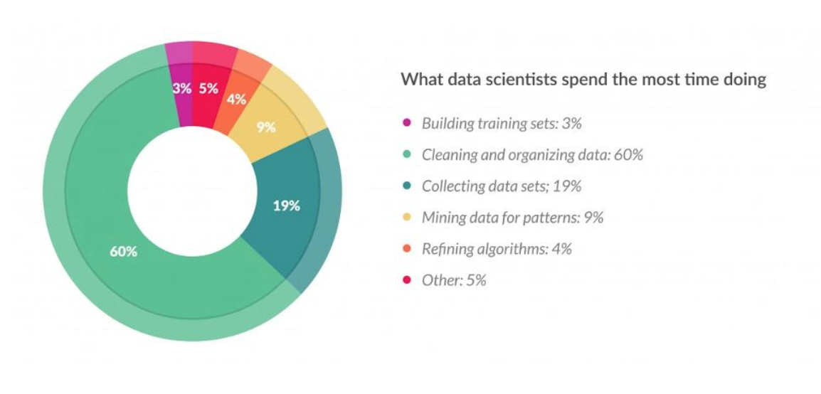
This is the survey from data scientists. You can find out this work will be unpleasure, takes lot of time, but also shows the importance of this work.
I’ll add on some pre-processing logic in data which I worked on previous post, to see how this process makes change.
Data transform
Look values in Name column, and you could find there are additional title such as ‘Mr’, ‘Mrs’, ‘Sir’, ‘Dr’, or else. By this data, you could assume target’s gender or position. Because this is story of early 20 century, which was hierarchical society, so we could estimate this could have relation with survival rate. Let’s add new column Title to use this.
{% highlight python %} {% raw %} train_df[‘Title’] = train_df[‘Name’].str.extract(’([A-Za-z]+).’) pd.crosstab(train_df[‘Title’], train_df[‘Sex’]) {% endraw %} {% endhighlight %}

Now column Title keeps parsed value from name, but there are bit varied so need to wrap similar values. Purpose for this column is to find out relation between ’title’ and ‘survival’ so I’ll wrap values with new name by its rank.
Also, unify value of different spelling but has similar meaning, such as ‘Mlle’ and ‘Ms’ which all can be equal with ‘Miss’.
- ‘Capt’, ‘Col’, ‘Don’, ‘Dr’, ‘Major’, ‘Rev’, ‘Jonkheer’, ‘Dona’ => Rare(others)
- ‘Countess’, ‘Lady’, ‘Sir’ => Royal(people of high standing)
- ‘Mlle’, ‘Ms’ => Miss
- ‘Mme’ => Mrs
Now redefine value of Title, and compare survival rates by this.
{% highlight python %} {% raw %} train_df[‘Title’] = train_df[‘Title’].replace([‘Capt’, ‘Col’, ‘Don’, ‘Dr’, ‘Major’, ‘Rev’, ‘Jonkheer’, ‘Dona’], ‘Rare’) train_df[‘Title’] = train_df[‘Title’].replace([‘Countess’, ‘Lady’, ‘Sir’], ‘Royal’) train_df[‘Title’] = train_df[‘Title’].replace([‘Mlle’, ‘Ms’], ‘Miss’) train_df[‘Title’] = train_df[‘Title’].replace(‘Mme’, ‘Mrs’) train_df[[‘Title’, ‘Survived’]].groupby([‘Title’], as_index=False).mean() {% endraw %} {% endhighlight %}
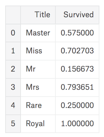
Survival rate of people with title ‘Miss’/‘Mrs’, who are female, appears high, as we look before. And also, who has title ‘Royal’/‘Master’, that we could assume high-positioned people, also survived more than others. So we could define as ‘people’s rank is related with survival rate’.
Missing value treatment - Age
There are some ways for treating missing values
- Delete
- Replace with mean or mode value
- Replace with estimated value using regression or else
- etc.
In this post, I’ll go on with 2, but not just fill mean value of all data in all missing data. I’ll work with assumption:
People who has same
Titlewill be in same age group.
So first look on mean value of age by Title.
{% highlight python %}
{% raw %}
train_df.groupby(‘Title’)[‘Age’].mean()
{% endraw %}
{% endhighlight %}
…it will be: {% highlight shell %} {% raw %} Title Master 4.574167 Miss 21.845638 Mr 32.368090 Mrs 35.788991 Rare 45.894737 Royal 43.333333 Name: Age, dtype: float64 {% endraw %} {% endhighlight %}
Now fill in value to missing data. {% highlight python %} {% raw %} train_df.loc[(train_df[‘Age’].isnull())&(train_df[‘Title’]==‘Master’),‘Age’] = 5 train_df.loc[(train_df[‘Age’].isnull())&(train_df[‘Title’]==‘Miss’),‘Age’] = 22 train_df.loc[(train_df[‘Age’].isnull())&(train_df[‘Title’]==‘Mr’),‘Age’] = 33 train_df.loc[(train_df[‘Age’].isnull())&(train_df[‘Title’]==‘Mrs’),‘Age’] = 36 train_df.loc[(train_df[‘Age’].isnull())&(train_df[‘Title’]==‘Rare’),‘Age’] = 45 train_df.loc[(train_df[‘Age’].isnull())&(train_df[‘Title’]==‘Royal’),‘Age’] = 43 {% endraw %} {% endhighlight %}
Data binning - Age
The case we are looking is binary classification, as there are only two label for result(live or die). In this case, continuous data needs to be grouped as category to deduct classifed result.
Data binning is a process wraping continuous data with group by specific criteria. My rule is:
- Less than 7 : Baby & Kids (0)
- 8~20: Students (1)
- 21~30: Young Adults (2)
- 31~40: Adults (3)
- 41~60: Seniors (4)
- More than 60: Elders (5)
I’ll make a column AgeGroup, and update these value.
{% highlight python %}
{% raw %}
train_df[‘AgeGroup’] = 0
train_df.loc[ train_df[‘Age’] <= 7, ‘AgeGroup’] = 0
train_df.loc[(train_df[‘Age’] > 7) & (train_df[‘Age’] <= 18), ‘AgeGroup’] = 1
train_df.loc[(train_df[‘Age’] > 18) & (train_df[‘Age’] <= 30), ‘AgeGroup’] = 2
train_df.loc[(train_df[‘Age’] > 30) & (train_df[‘Age’] <= 40), ‘AgeGroup’] = 3
train_df.loc[(train_df[‘Age’] > 40) & (train_df[‘Age’] <= 60), ‘AgeGroup’] = 4
train_df.loc[ train_df[‘Age’] > 60, ‘AgeGroup’] = 5
f,ax=plt.subplots(1,1,figsize=(10,10))
sns.countplot(‘AgeGroup’,hue=‘Survived’,data=train_df, ax=ax)
plt.show()
{% endraw %}
{% endhighlight %}
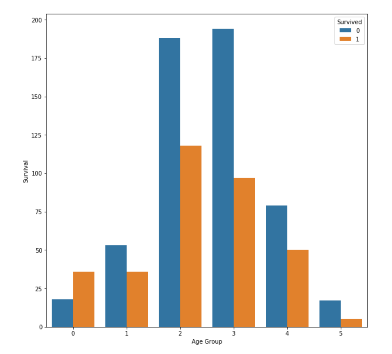
People in group 0(Baby & Kids) has high survival rate, while other groups looks same. We can think that elder people make way to live to yongsters.
Outlier, and data binning - Family member
There are also data which defines family members, SibSp(Sibling & Spouse) and Parch(Parent & children). In my mind, priority of both are same, so I’ll merge these 2 into new column FamilyMember.
{% highlight python %} {% raw %} train_df[‘FamilyMembers’] = train_df[‘SibSp’] + train_df[‘Parch’] + 1 pd.crosstab([train_df[‘FamilyMembers’]],train_df[‘Survived’]).style.background_gradient(cmap=‘summer_r’) {% endraw %} {% endhighlight %}
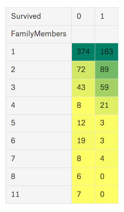
Something weird is, there are 7 people wrote as they are with 11 family member, and it means at least 4 people wrote wrong number. So you could think there are several ‘outlier’ in this data. So I’ll not use this column directly, but create new one based on this data with rule:
‘Existence’ of family member would be important, more than the number.
because family member should help each other(maybe not…) to survive. New columne IsAlone is defined as 0 if it has family member, else 1.
{% highlight python %} {% raw %} train_df[‘IsAlone’] = 0 train_df.loc[train_df[‘FamilyMembers’] == 1, ‘IsAlone’] = 1 f, ax=plt.subplots(1,2,figsize=(20,8)) ax[0].set_title(‘Survived, with family’) train_df[‘Survived’][train_df[‘IsAlone’]==0].value_counts().plot.pie(explode=[0,0.1],autopct=’%1.1f%%’,ax=ax[0],shadow=True) train_df[‘Survived’][train_df[‘IsAlone’]==1].value_counts().plot.pie(explode=[0,0.1],autopct=’%1.1f%%’,ax=ax[1],shadow=True) ax[1].set_title(‘IsAlone Survived’) plt.show() {% endraw %} {% endhighlight %}
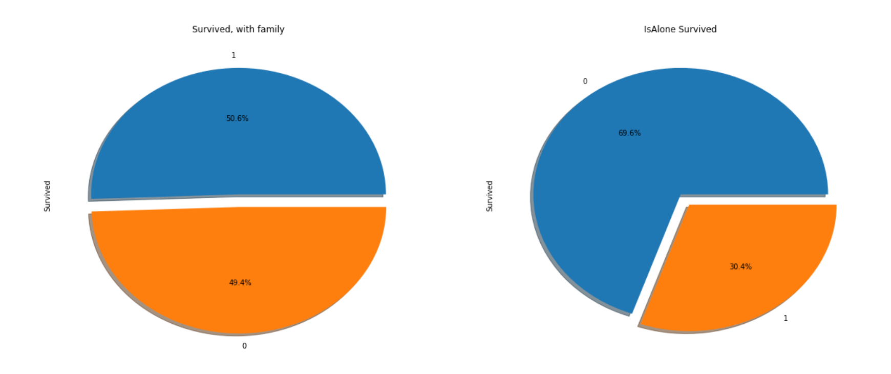
As assumed, people with family’s survival rate(50%) was higher than who is alone(30%).
Modeling with pre-processed data
It used same modeling algorithm with previous result(Decision tree), but add columns we generated in this post, TitleKey, AgeGroup and IsAlone.
{% highlight python %} {% raw %} train, test = train_test_split(train_df,test_size=0.3,random_state=0) target_col = [‘Pclass’, ‘Sex’, ‘Embarked’, ‘TitleKey’, ‘AgeGroup’, ‘IsAlone’] train_X=train[target_col] train_Y=train[‘Survived’] test_X=test[target_col] test_Y=test[‘Survived’] features_one = train_X.values target = train_Y.values tree_model = DecisionTreeClassifier() tree_model.fit(features_one, target) dt_prediction = tree_model.predict(test_X) print(‘The accuracy of the Decision Tree is’,metrics.accuracy_score(dt_prediction, test_Y)) {% endraw %} {% endhighlight %}
The result of accuracy is 0.813432835821, bit higher than before(0.809701492537).
Actually in pre-processing, as much as understanding algorithm, you need to have knowledge about period/situation when data occured. By knowing the background, you can make data more closer to the real world. So for good data research, you need to think about ‘story’ of the data and having imagination from it based on situation.