Starting neural network with tensorflow

It has been several years since deeplearning became common in our life. Lots of services are based on it, and you can find guide books/documents easily in bookstore or google. But it is hard to go on deeply by understanding theories and logics, for most of engineer who is not majored this. Though I’m working on deep learning company(as a web engineer), still suffering with its principle and mathematical formulas. This note, is the challenge for going with this from basic.

Tensorflow, and deep learning libraries

Though you are not a deep learning engineer, you would heard about tensorflow. Since google released as open source on 2015, it has been most popular deep learning libraries. Somebody could just think it is the power of google brand, but it is really a thing. It has well-designed APIs, good documents translated with various languages, and most important, it is being used in lots of real world service including google photo, google translate, gmail, android, and more.

Now other major IT companies(Facebook, Microsoft, Amazon…) are releasing their deep learning libraries as open source, and competiting with tensorflow. It’s good news for engineers having lot of options. But I think it is meaningless thinking which option you will select, if you are not used to on logic of how deep learning are working on and how to use it. So I’ll only deal with tensorflow here. As I said, I’m really a beginner in deep learning yet.

Artificial Neural network

If you heard of deep learning, you would also heard about artificial neural network(ANN). As you could expect in word ‘artificial’, it is something imitate neural network in human brain to replicate how human learns from data.

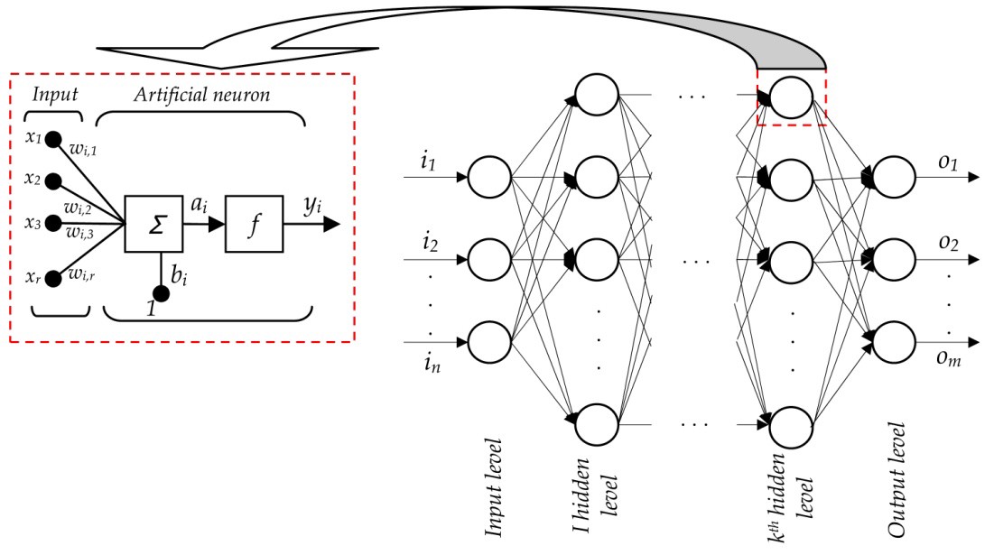
This is basic form of ANN. There are input layer, hidden layer(can be more than 1), and output layer. These layers are made of nodes, which are workin as neuron in human. Each node receives multiple data, calculate based on some function, and send result to connected nodes.

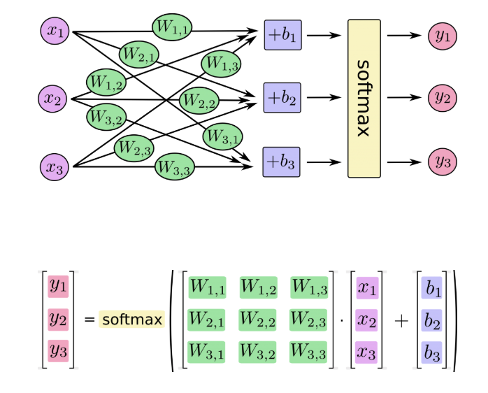
With input, weight and bias, by logistic regression logic, it will return the rate of possibility that which class input is. Softmax regression is, one general regression logic, which normalize return values to make sum value as 1. Truely, actual logic is way more complicate, but I’ll not discuss here. It will need a textbook to write it all.

Hope on to the example.

Setup for research

First, import tensorflow library, and image data for research. I’ll use fashion-mnist data, 60,000 imageset of clothing/shoes. Each of them are 28x28 grayscale image, classified to 10 classes. Data includes label list of class, as below.

You can download dataset here.

 1
 2
 3
 4
 5
 6
 7
 8
 9
10
11
12
13
14
15

import tensorflow as tf
from tensorflow.examples.tutorials.mnist import input_data
fashion_mnist = input_data.read_data_sets("path/of/fashion-mnist", one_hot=True)
class_names = [
    'T-shirt/top',
    'Trouser',
    'Pullover',
    'Dress',
    'Coat', 
    'Sandal',
    'Shirt',
    'Sneaker',
    'Bag',
    'Ankle boot'
]

Import tensorflow module, and datasets to your project. By using tensorflow.examples.tutorials.mnist.input_data, you can receive data as tensorflow DataSet object from formatted zip files. This DataSet type offers APIs to make training code more simple. Labels are defined as 0 to 9 as we saw on table above. So let’s set as a name in class_name array.

Now check received data. It has 2 DataSet as train and test. Each of it includes 2-dimension numpy array, including information of dataset.

1
2
3
4

fashion_mnist.train.images.shape    #(55000, 784)
fashion_mnist.train.labels.shape    #(55000, 10)
fashion_mnist.test.images.shape     #(10000, 784)
fashion_mnist.test.labels.shape     #(10000, 10)

Each image data are composed as an array with 784 formula. It is data of each pixel in 28x28(=784) image. Labels are more simple, it is just array with 10 formula, which defines what kind of image(class) it is.

Than let’s look on few data.

 1
 2
 3
 4
 5
 6
 7
 8
 9
10
11

import matplotlib.pyplot as plt

fig = plt.figure(figsize=(8, 8))
for i in range(4):
    target_train_num = i + 5
    fig.add_subplot(2, 2, i+1)
    plt.imshow(fashion_mnist.train.images[target_train_num].reshape(28, 28), cmap='Greys')
    label_num = np.where(fashion_mnist.train.labels[target_train_num] == 1)[0][0]
    print(class_names[label_num])
    
plt.show()

This picks 5th to 8th data, and show label name and image. Because image is defined as 1d array, I changed to 28x28 2d array.

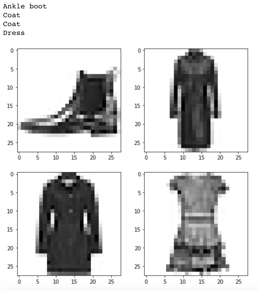
Okay, data seems good. Let’s look on the logic bit more.

Entropy, and Cross-entropy

Surprisal analysis is one technique of Information theory, which calculates the degree/amount of ‘surprised’ by getting certain information. In formula, it can be show as

For example, let’s say I have 2% possibility of winning the lottery. In this case:

• Winning the lottery => log(1/0.02) = 1.69897000434
• Not winning the lottery => log(1/0.98) = 0.0087739243

In information theory, it assume ‘degree of uncertain event’ is larger than certain ones. By this theory, it shows the surprisal degree of getting information ‘winning lottery’ is almost 200 times larger than the other case.

Okay, now go with Entropy(a.k.a ‘Shannon Entropy’). This is mean value of this ‘surprisal’ in one event. It is defined as:

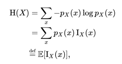
In case above, it can described as => (0.98 x 0.0087739243) + (0.02 x 1.69897000434)

We can say Entropy of my lottery game is 0.04256.

But because we cannot expect the future, this can be known after when lottery game is ended. So what we need to see is Cross-Entropy. By this name, we could think it is some kind of combining logic between Entropy. Let’s think the actual probability as ‘p’, and estimated probability is ‘q’. In this situation, we need to make ‘q’ close to ‘p’. In information theorical way, Cross-Entropy means ‘average number of bits needed to identify an event drawn from the set’. More simple, it can be said ’the range between expected / actual event’.

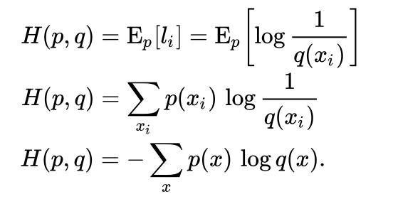
This formula will return larger value as this ‘range’ become longer. It means we need to think of reducing this value, to make expectation as close as the real one. There are lot of functions for this, but I’ll use Gradient Descent algorithm here, which are usually used for basic tutorial.

Let’s get back to source.

Making layers, and training in TF

1
2
3
4
5
6
7
8
9

...
X = tf.placeholder(tf.float32, [None, 784])
W = tf.Variable(tf.zeros([784, 10]))
b = tf.Variable(tf.zeros([10]))
k = tf.matmul(X, W) + b

y = tf.nn.softmax(k)
y_ = tf.placeholder(tf.float32, [None, 10])
...

This is to make input placeholder for network. X is 784 dimension vector to put in image data. W and b means weight and bias. Model’s variable in tensorflow usually defined as Variable.

1
2

cross_entropy = tf.reduce_mean(tf.nn.softmax_cross_entropy_with_logits_v2(labels=y_, logits=k))
cost = tf.train.GradientDescentOptimizer(0.05).minimize(cross_entropy)

First line is to normalize inputs, and generate the result with Cross-Entropy. Thankfully, Tensorflow offer APIs to make it with single line. Also for Gradient Descent, it can be implemented simply with this.

 1
 2
 3
 4
 5
 6
 7
 8
 9
10
11
12
13
14
15
16
17
18

init = tf.global_variables_initializer()
sess = tf.Session()
sess.run(init)

epochs = 10
batch_size = 100
total_batch = int(fashion_mnist.train.num_examples / batch_size)
    
for epoch in range(epochs):
    total_cost = 0

    for i in range(total_batch):
        batch_xs, batch_ys = fashion_mnist.train.next_batch(batch_size)

        _, cost_val = sess.run([cost, cross_entropy], feed_dict={X: batch_xs, y_: batch_ys})
        total_cost += cost_val
    
    print('Epoch:', '{:d}'.format(epoch), 'Cost =', '{:.5f}'.format(total_cost / total_batch))

batch_size means how many training image will be used for single term. We can get data of batch size with train.next_batch API which are offered by Tensorflow DataSet. It is returning random value from data source, so we don’t need additional code for this.

Epoch means the number of training total data. It has been setup as 10. Because data is always being trained with random order, the cost(mimimized result by Gradient Decsent) will become lower by training term.

Epoch: 0 Cost = 0.75573
Epoch: 1 Cost = 0.55515
Epoch: 2 Cost = 0.51330
Epoch: 3 Cost = 0.49104
Epoch: 4 Cost = 0.47568
Epoch: 5 Cost = 0.46544
Epoch: 6 Cost = 0.45749
Epoch: 7 Cost = 0.45073
Epoch: 8 Cost = 0.44577
Epoch: 9 Cost = 0.44050

Result, and still more things need to know.

Now we can compare trained result with test data.

1
2
3
4

correct_prediction = tf.equal(tf.argmax(y,1), tf.argmax(y_,1))
accuracy = tf.reduce_mean(tf.cast(correct_prediction, tf.float32))
sess.run(accuracy, feed_dict={X: fashion_mnist.test.images, y_: fashion_mnist.test.labels})
# 0.8362

It returns 0.8362. Seems not good enough, but nevermind. It is not the purpose here. This is just note for basic understanding.

Though I write over about this until now, still lot of things are uncomprehended.

• What is difference between softmax_cross_entropy_with_logits and softmax_cross_entropy_with_logits_v2?
• How does tuning the value of GradientDescentOptimizer effects the result?
• Is there other optimizer, and what are the pros and cons of them?
• How nunber of ‘batch’ and ’epoch’ effect to the result?
• and more…

I’ll keep look on this with next post for deeplearning and Tensorflow.

References

• https://www.tensorflow.org/tutorials/
• https://hackernoon.com/artificial-neural-network-a843ff870338
• https://www.digitalocean.com/community/tutorials/how-to-build-a-neural-network-to-recognize-handwritten-digits-with-tensorflow
• https://github.com/zalandoresearch/fashion-mnist
• https://ml-cheatsheet.readthedocs.io/
• https://en.wikipedia.org/wiki/Information_content
• https://en.wikipedia.org/wiki/Cross_entropy
• https://medium.com/@vijendra1125/understanding-entropy-cross-entropy-and-softmax-3b79d9b23c8a